sobol_algorithm

This function calculates the Sobol-sensitive indexes for any function using sampling. This function computes the first-order and total-order Sobol indexes.

data_sobol = sobol_algorithm(setup)

Input variables

Name	Description	Type
setup	A dictionary containing the settings for the numerical model and analysis. 'number of samples': Number of samples [Integer] 'numerical model': Numerical model settings [Dictionary] 'variables settings': Variables settings, listed as dictionaries [List] 'number of state limit functions or constraints': Number of state limit functions or constraints [Integer] 'none_variable': Generic variable for use in the objective function [None, List, Float, Dictionary, String, or other type] 'objective function': Objective function defined by the user [Python function]	Dictionary

Output variables

Name	Description	Type
data_sobol	A dictionary containing the first-order and total-order Sobol sensitivity indixes for each input variable.	Dict

Example 1

This example demonstrates how to use the `sobol_algorithm` function to calculate the Sobol indixes for a structural reliability problem.

Due to its nonlinear properties and variable interactions, the Ishigami function is commonly used as a test function for comparing global sensitivity analysis methods. This function is particularly valuable for benchmarking different sensitivity analysis methods, making it a classic example.

The function takes as input a vector \( x = [x_0, x_1, x_2] \), which represents three independent variables. Its analytical expression is defined as:

\[f(x) = \sin(x_0) + a \cdot \sin^2(x_1) + b \cdot x_2^4 \cdot \sin(x_0)\]

where:

• \( x = \{x_0, x_1, x_2\}\) are the input variables, uniformly distributed in \([-\pi, \pi]\);
• \( a \) and \( b \) are adjustable parameters that control the relative impact of each term in the function. We use \( a=7.00 \) and \( b=0.10 \).

of_file.py

def ishigami(x, none_variable):
    """Objective function for the Nowak example (tutorial).
    """
    a = 7.00
    b = 0.10
    # Random variables
    x_0 = x[0]
    x_1 = x[1]
    x_2 = x[2]
    result = np.sin(x_0) + a * np.sin(x_1) ** 2 + b * (x_2 ** 4) * np.sin(x_0)

    return [None], [None], [result]

How the Sobol algorithm leverages the sampling_algorithm_structural_analysis is necessary assemble objective function using same pattern that this function. See example (of_file)[sampling_algorithm_structural_analysis]. Put your function in last return.

your_problem.ipynb

from parepy_toolbox import sobol_algorithm

# Dataset
f = {'type': 'uniform', 'parameters': {'min': -3.14, 'max': 3.14}, 'stochastic variable': False}
p = {'type': 'uniform', 'parameters': {'min': -3.14, 'max': 3.14}, 'stochastic variable': False}
w = {'type': 'uniform', 'parameters': {'min': -3.14, 'max': 3.14}, 'stochastic variable': False}
var = [f, p, w]

# PAREpy setup
setup = {
             'number of samples': 50000, 
             'number of dimensions': len(var), 
             'numerical model': {'model sampling': 'lhs'}, 
             'variables settings': var, 
             'number of state limit functions or constraints': 1, 
             'none variable': None,
             'objective function': ishigami,
             'name simulation': None,
        }

# Call algorithm
data_sobol = sobol_algorithm(setup)

How the Sobol algorithm leverages the sampling_algorithm_structural_analysis is necessary assemble setup variable using same pattern that this function. See example (setup file)[sampling_algorithm_structural_analysis].

Post-processing

Show all results

How do we display the Sobol indices calculated for the Ishigami function?

# Show results in notebook file (use the dictionary's variable name in the code cell)
data_sobol

# or 
# Show results in Python file (using the print function)
print(data_sobol)

Output details:

+----+-----------+----------+
|    |       s_i |      s_t |
|----+-----------+----------|
|  0 | 0.312931  | 0.547654 |
|  1 | 0.44652   | 0.433496 |
|  2 | 0.0097489 | 0.220905 |
+----+-----------+----------+

• s_i: First-order Sobol index, representing the individual contribution of the variable to the output variance.
• s_t: Total-order Sobol index, representing the overall contribution, including interactions with other variables.

Plot results

How do we visualize the Sobol indices as bar charts to interpret the results?

# Libraries
import matplotlib.pyplot as plt

# Extract values
variables = ['x_0', 'x_1', 'x_2']
s_i = [data_sobol.iloc[var]['s_i'] for var in range(len(variables))]
s_t = [data_sobol.iloc[var]['s_t'] for var in range(len(variables))]

# Plot bar chart for Sobol indixes
x = range(len(variables))
width = 0.35
plt.bar(x, s_i, width, label='First-order (s_i)', color='blue', alpha=0.7)
plt.bar([p + width for p in x], s_t, width, label='Total-order (s_t)', color='orange', alpha=0.7)
plt.xlabel("Variables")
plt.ylabel("Sobol Index")
plt.xticks([p + width / 2 for p in x], variables)
plt.legend()
plt.show()

Output details:

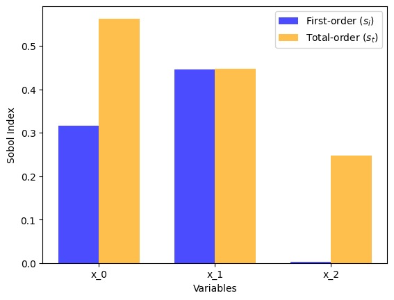
Figure 1. Sobol indices for the Ishigami function.

Save results to a file

To save the Sobol indices for further analysis or reporting:

# Save results to a CSV file
data_sobol.to_excel('sobol_indices.xlsx', index=False)

print("Sobol indices saved to 'sobol_indices.xlsx'")